Hypothesis: It is possible, in at least in some straightforward cases, to populate a CNN-like structure with a state that is intelligible from an analysis point of view.

1 Introduction

Currently, the state-of-the-art (SOTA) approach for image classification is Convolutional Neural Networks (CNN) [10]. Unfortunately, the impressive performance of a CNN comes at a cost; its underlying model is essentially a black box [11] (meaning that it is generally unintelligible to humans). This makes it challenging to evaluate CNN systems for correctness. It can also be quite difficult to reuse, debug, or update the models of CNN systems.

This article is the first in a series of investigations to discover the qualities that make CNN systems such an effective tool for classification. If some (or all) of the CNN “secret sauce” is found, the next challenge could be to transfer this into a significantly more intelligible system. Our approach (across multiple articles) will involve implementing increasingly complicated CNN explanatory models that can then be compared to the performance of actual CNN systems to determine their validity. If high performance can be achieved using an explanatory model, this will go a long way towards achieving the goal of a high-quality intelligible state machine learning system.

Naturally, the core focus of our solution will be on its transparency (a solution with intelligible internal states), with the idea that this will be useful for formulating clear explanations as to why the proposed ideas are working or failing.

Finally, it should be pointed out that this article often refers to the notion of a feature in images. In this context, a feature is some sub-pattern within images. This can be a small local pattern, such as a corner, or something more complex and abstract, such as the pixels of high response when a software frequency filter is applied to the image data.

2 Problem Description

As the focus of this article is on image classification CNN systems, it was necessary to choose a suitable problem. A key attribute of this problem was its simplicity, as the goal of this work is analysis and complexity hampers analysis.

While there are many viable options, the problem of discriminating between images of triangles and images of squares was the one that was selected for this work (with the main rationale being that corner features seemed intuitive to focus on, and both squares and triangles have corners). It was decided to make the images “black and white” to avoid extra complexity around color. To add variety, the images were rotated about the center and scaled (with a variance of about 10 pixels) to have subtly different sizes (both choices were arbitrary). The images were $210 \times 210$ pixels (again, this number was arbitrarily selected).

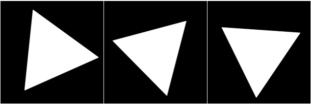
Figure 1: A selection of the various triangle images within the database.

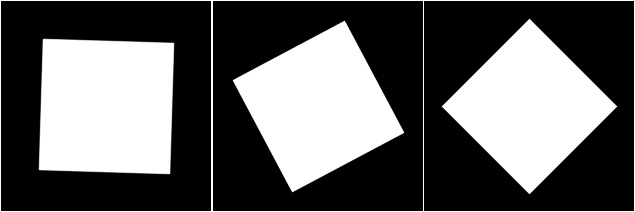
Figure 2: A selection of the various square images within the database.

Several approaches exist to solving such a problem (using traditional computer vision techniques). One approach would be a “whole image” template matching with rotation invariance [5]. Other strategies involve discovering features within images such as edges [15] or corners [13] and using the feature count as a discriminator.

3 Methodology

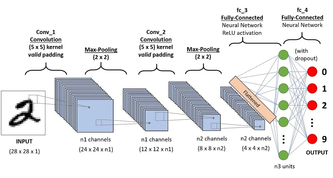
Figure 3: A Convolutional Neural Network (CNN) for image classification.

Figure 3 depicts the structure of a typical CNN for image classification. This is the structure whose internal state we are trying to “explain”. It takes an image to be classified as an input and outputs a classification. The processing to arrive at the classification begins by passing the image through several layers of convolutional filters (explained below). Each layer applies several filters to the image to produce several responses. This set of responses is then combined and sub-sampled (preserving the most prominent outputs from filtering) into a singular result for the layer. As the image proceeds down the layers, it becomes increasingly smaller with increasingly more complex compound filter responses. The final output is then flattened (converted to a 1D vector) to serve as an image descriptor. This descriptor is then passed to a traditional (fully connected) artificial neural network (ANN), which performs the final classification.

The weights that comprise the convolutional filters and nodes in the ANN are acquired during training (the processing of fitting the model to a sample dataset) through a process known as back-propagation. Back-propagation is a process of propagating errors down the network layers to correct weights contributing to those errors.

Our implementation aims to attempt to maintain the structure of the CNN depicted in figure 3 but to formulate it so that the model’s internal state is intelligible. To control the internal state, we will attempt to manually populate the state with a solution rather than using the traditional training with back-propagation processes to achieve this.

This section has been split into two subsections: Section 3.1 outlines the steps that we have made to make our model intelligible. Section 3.2 then outlines how the state was configured to perform classification.

3.1 Make it Explainable

This section covers modifications we made to the typical CNN structure to make the internal state of the network more explainable. Two main changes were made. The first was to convert the convolution filters into matching templates. The second was to replace the ANN at the end of the process with a more “transparent” classifier.

3.1.1 Convolution Filtering

Figure 3 shows that the first layers of the classifier are banks of convolution filters [14]. What is convolution? It is a mathematical operation. The operation “applies” a filter $F$ to a signal $S$, and has the effect of boosting some frequency signals and dampening others. The filter $F$ is called a filter because its traditional context is signal processing, where it is used to “filter out” some of the frequency range, for example, high-pass filters and low-pass filters. Convolution also has become popular in image processing [9], where the image $I$ data is viewed as a 2D signal, in which spatial dimensions have been substituted for time dimensions. Since images $I$ are discrete entities (indexed by discrete pixels), the formulation for convolution in image processing is typically converted to a discrete form, such as

\[[F * I](u,v) = \sum_{i=-k}^k \sum_{j=-k}^k F(i,j)I(u-i,v-j) \ \ \ \ [1]\]

The symbol for the convolution operation is $*$. Equation 1 specifies that given the convolution $F * I$ between filter $F$ and image $I$, the response at pixel $[u,v]^{\top}$ is the sum of the weights in filter $F$ at location $[i,j]^{\top}$ multiplied by corresponding pixels $[u-i, v-j]^{\top}$ in the image $I$ in the range of $[-k,k]$ for both $i$ and $j$.

In image processing, the $F$ resembles a small “image” (a single channel 2D array of weights), and the chosen weights determine the filter’s filtering effect on the image $I$. For example, one such filter $F$ is called the Sobel filter $F_s$ (see figure 4).

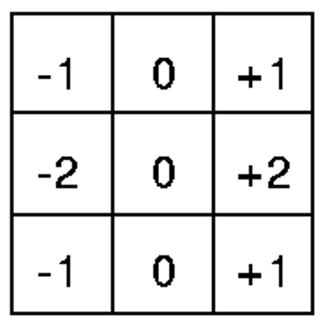
Figure 4: A Sobel filter for detecting high-frequency changes in the x-direction within an image. It is formulated as a 2D array of weights.

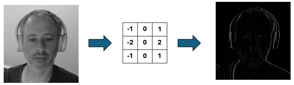
Figure 5: An example of the x-direction Sobel filter response after convolution. The image on the left is the original, the center shows the filter, and the right shows the response.

The main problem with convolution filters is that the filter’s effect is not always immediately apparent from the filter $F$ itself (see figure 6). Naturally, there are ways of establishing the impact, such as applying the filter $F$ to the image $I$ to see what “it does”. Or one could determine the response in the frequency domain by calculating the Fourier Transform [12].

However, it would be great to achieve this by observing the filter $F$, which is often unclear unless the observer has seen enough filters to start using their experience to predict outcomes.

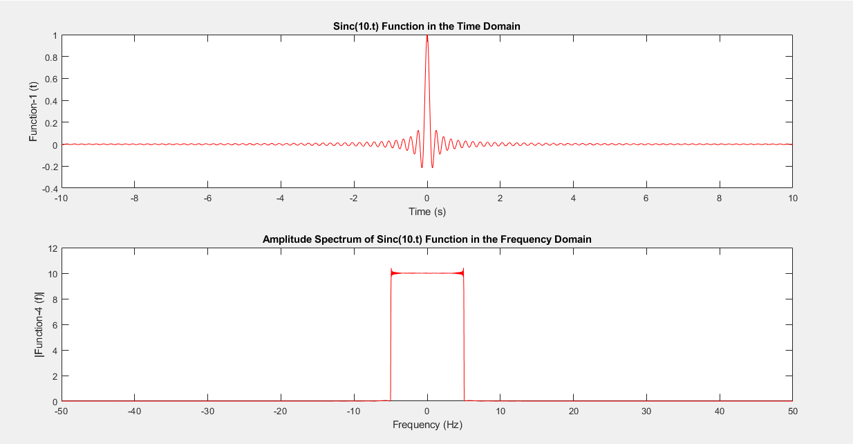
Figure 6: The sinc function ($sinc(x) = sin(x) / x$). In the context of convolution, this filter is called the “box filter”. In the figure, the sinc function is plotted at the top, and its response in the frequency domain is plotted at the bottom. When applied to a convolution signal, the frequencies are only retained in a particular range. However, this is typically not immediately obvious to the novice observer when looking at the function.

The solution proposed in this article is to try and find an alternative approach to filtering that achieves the same goal. The convolutional filters’ operation in a CNN is postulated to be feature extraction (features are defined in section 2). Therefore, we are looking for an alternative “filtering” approach that extracts features from images but operates in the image domain rather than the frequency domain (convolution filters are obscure because they operate in a “different” domain).

It turns out that convolutional is quite similar to another operation called cross-correlation. The formulation for cross-correlation is as follows

\[[F \otimes I](u,v) = \sum_{i=-k}^k \sum_{j=-k}^k F(i,j)I(u+i,v+j) \ \ \ \ [2]\]

The symbol for the cross-correlation operation is $\otimes$. As can be seen, in comparison to equation 1, equation 2 is almost the same, except that the order of the pixels being multiplied together is reversed.

Cross-correlation is also used in image processing. However, it is used in template matching [4]. Template matching is when a larger image is expected to contain a smaller sub-image (called a template). The process is a systematic search in which the template is placed at each pixel within the image, and a score is calculated based on how well the template matches the local neighborhood of the pixel. If the score is within some threshold, a match is recorded. See figure 7.

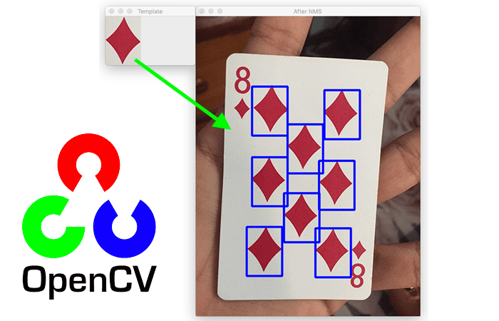
Figure 7: An illustration of template matching. Here, the “template” is an image of a diamond. Each pixel within the image is systematically checked to see how well the template “fits” in that location. Areas of good fit are recorded as matches.

In template matching, the template has a similar form to the convolutional filter. However, here they are preferred since they “look” like the feature they match. Note that cross-correlation can be considered to be one type of cost function used for template matching; others are the Sum of Square Differences (SSD) and the Sum of Absolute Differences (SAD).

3.1.2 Classification Logic

As previously noted, the first part of the CNN is a set of convolutional filter layers that transform an image into a feature-based image descriptor. In the previous section section 3.1.1, we proposed replacing this set of convolutional filters with layers of template matching.

The next part of the network uses the extracted image descriptor to classify the image. A standard Artificial Neural Network (ANN) is the usual tool for achieving this. However, the fact that an ANN is a “black box” goes against the spirit of this work. Fortunately, there exists a set of more transparent machine-learning algorithms, including Bayesian Learning [4], Rule-base learning [6] and Decision Trees [8]. The downside of these approaches is that they are often too simplistic to encode complicated models. However, for the problem at hand, it is felt that at least one of these approaches should be able to serve the purpose.

3.2 Setting up the state

In section 3.1, modifications to the traditional CNN were introduced to make the internal state more explainable. A disadvantage of the new formulation is that it is less straightforward to fit models to data (something we will address in future work). In the case of a CNN, this is typically achieved by stochastic gradient descent [1].

Concerning the problem of shape detection, it was felt that the state was intuitive enough to assemble a solution “by hand”. The most notable feature of the two shapes (square and triangle) is the notion of a corner. As per section 3.1.1, we have adjusted our formulation of a feature to be able to represent a corner explicitly - simply as an image of a corner. Scores can be calculated using cross-correlation. Figure 8 shows an example of calculating a response image of a triangle, given a corner feature. In this example, we used the SSD cost function (instead of pure cross-correlation) and a color inversion (swap light and dark colors) to improve the response image’s visual intuition further.

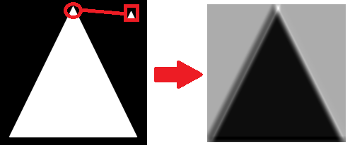
Figure 8: On the left, a corner feature is matched (in the red block) to the image of a triangle. On the right is a “heat map” containing match scores, with black indicating a low score and white indicating a good match.

Of course, as seen in figure 8, the single-corner feature is only helpful in detecting one of the shape’s corners. So, to account for the fact that a triangle has three corners, and the dataset consists of an entire array of orientations, the same corner was added to a filter bank $360$ times, with each rotated to a different angle in the discrete $360^{\circ}$ range. A visualization of this can be seen in figure 9.

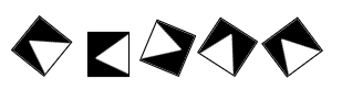
Figure 9: A sampling of corner features at different orientations, used in the filter bank.

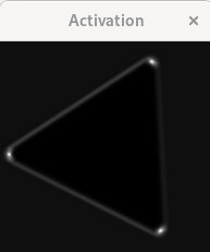
Figure 10: The final activation map from a feature bank of $360$ corner images containing the best responses. SSD scoring was used, and the values were inverted. The score $s$ was remapped to $s’ = e^{- \alpha s}$ to emphasize the areas of high response. Here $\alpha$ is a scaling factor.

Matching the $360$ corner features to a single image in the problem dataset produces $360$ response images. These responses can then be combined into a single image. This is achieved by setting each pixel to the best score for that pixel from the entire set of activation images. The result can be visualized, as shown in figure 10.

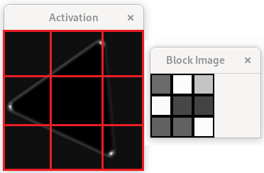
Figure 11: On the left is the final activation map, with an overlaid grid of $9$ cells. The best value is then selected from each cell, making a $9$ value descriptor of the image, visualized on the right as a $3 \times 3$ grid with the intensity of the best response coloring the corresponding cell.

To compress this into an image descriptor, the next step was to divide the final activation map into a grid of $9$ cells. Each cell represents a variable and is populated with the value of the best response in that cell. The process is illustrated in figure 11.

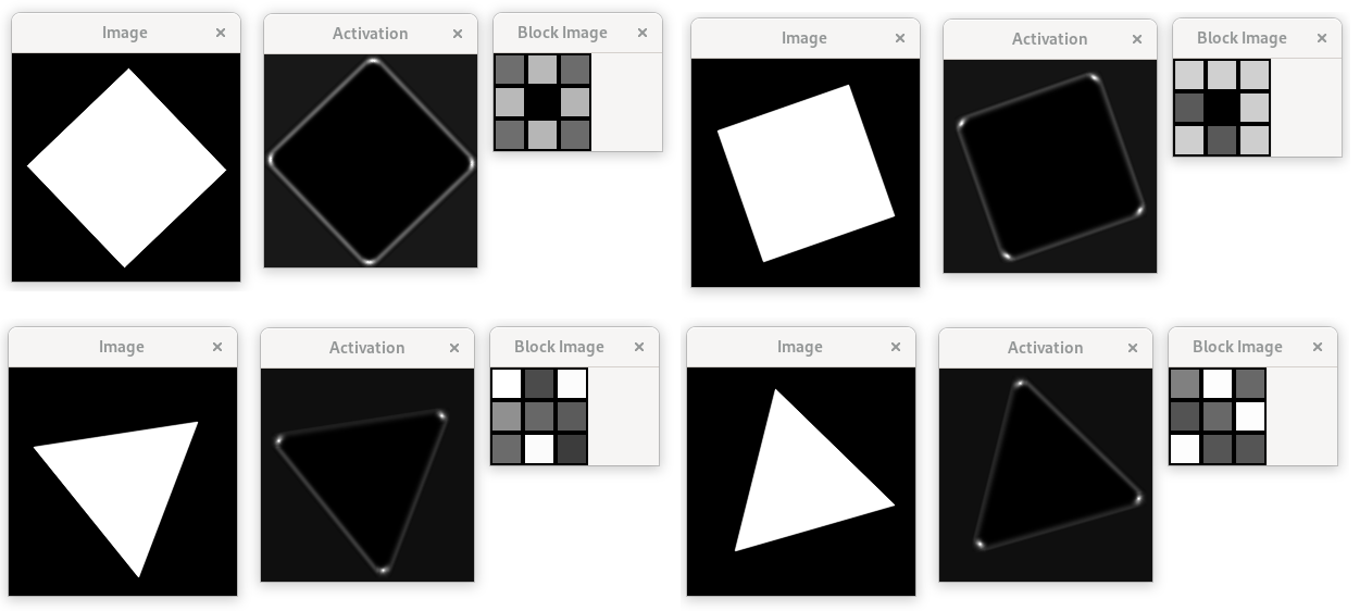
Figure 12: The final activation map and corresponding image descriptor vector for two triangle images and two square images.

Note that, as the problem being solved is relatively simple, only a single layer of filters is sufficient. However, “real-world” CNN systems that solve challenging problems typically contain several layers of filters.

As a final step, a rule-based is used to classify the image description. The rules for this were evolved using my Genetic Programming(GP), rule-based classifier [7].

4 Results

4.1 Timing

Given a $210 \times 210$ image with $360$ $10 \times 10$ features on a i7 processor at $3.00 \ GHz$, with $16.0 \ GB$ RAM. My implementation was a non-optimized C++ application that made use of OpenCV [2] library (version 4.20), which included the cv::matchTemplate() function. Testing was done using the Ubuntu 22.04 operating system.

Processing time per image was $0.48 \ ms$ with a standard deviation of $0.09 \ ms$.

4.2 Rule-Base classifier

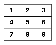
Figure 13: A map showing the indices of the attributes making up the index descriptor.

As mentioned at the bottom of section 3.2, a rule-based classifier was generated using Genetic Programming (GP). The classifier was trained to take an image descriptor as an input and produce a class (“triangle” [true] or “not triangle” [false]) as an output.

The above image, figure 13, indicates the numbering(indexes) variables in the image descriptor. As a convention, the index $i$ will be represented as ⓘ in our rule notion.

After training with $200$ training image descriptors (half in each class), the resultant rule model learned was as follows:

\[class = ⑤ > 50 \ \ \ \ [3]\]

The above rule model essentially learned that if the middle value ⑤ contained a matching value of above $50$, then the class was “true” (triangle); otherwise, it was “false” (square).

This rule exploited the fact that the center cell of images with squares was usually empty enough to have no feature in the middle (hence the low match score in the middle), while all the triangles typically had at least one edge overlapping the center cell, resulting in a higher match score. This can be visually verified in figure 12.

While this rule has utility, there was interest in whether the classifier could learn a rule that exploited the corner features more directly. Therefore another test was performed to see if the algorithm could “learn” a rule considering the corner features. Attribute ⑤ was removed from contention, and the algorithm was rerun. The resultant rule is as follows:

\[class = ① > 200 \lor ② > 200 \lor ③ > 200 \ \ \ \ [4]\]

In this context, if one of the attributes ①, ② or ③ had a high response (above $200$), then the class was “true” (triangle); otherwise, it was “false” (square). The “explanation” of this rule starts with the fact that triangle corners give a higher response than square corners (triangle ones are above $200$ while square corners are below). Given the triangle shape, it is noted that every configuration should have at least one corner on the top row.

So, in summary, two rules were generated by the GP training. Both rules were “transparent” models with clear explanations that are verifiable in the context of the problem.

4.3 Accuracy

Several accuracy tests were conducted with equation 3 and equation 4 with $5$ iterations of sets of $200$ “unseen” images. The final result was $100\%$ accuracy. This is not a surprising result, given the simplicity of the problem.

5 Conclusions

This work has focused on the internal state of Convolutional Neural Networks (CNN), which are notoriously unintelligible. The goal of this work was a first attempt to generate a CNN-like system with an intelligible internal state.

To achieve this, some modifications to the typical structure of a CNN were made. These were swapping out the convolutional filters, replacing them with template-matching “filters”, and replacing the Neural Network with a GP-learned rule-based model. The internal state, with regards to the filters, was manually set.

A classification problem was chosen for testing that was deliberately simple to facilitate the focus on an intelligible state.

The result of this work demonstrates that it is possible to formulate, given a simple enough problem, a CNN-like classifier with an internal state that could give technical users a clear insight into how the classifier operates. This intelligibility was maintained in both the filtering phase and the subsequent classification phase.

6 Future Work

This work is the first step in developing a system as effective as a CNN but with a more intelligible internal state. However, this solution does not scale to more challenging problems with complicated, noisy features. The next step of our journey is to investigate ideas around finding and matching complex features using an intelligible approach.

7 Reference

[1] Amari, Shun-ichi. 1993. “Backpropagation and Stochastic Gradient Descent Method.” Neurocomputing 5 (4-5): 185–96.

[2] Bradski, Gary. 2000. “The openCV Library.” Dr. Dobb’s Journal: Software Tools for the Professional Programmer 25 (11): 120–23.

[3] Briechle, Kai, and Uwe D Hanebeck. 2001. “Template Matching Using Fast Normalized Cross Correlation.” In Optical Pattern Recognition Xii, 4387:95–102. SPIE.

[4] Ch, Read, and ML MAP. 1997. “Bayesian Learning.” Book: Machine Learning. McGraw-Hill Science/Engineering/Math, 154–200.

[5] Fredriksson, Kimmo. 2001. “Rotation Invariant Template Matching.” PhD Thesis.

[6] Fürnkranz, Johannes, and Tomáš Kliegr. 2015. “A Brief Overview of Rule Learning.” In International Symposium on Rules and Rule Markup Languages for the Semantic Web, 54–69. Springer.

[7] Gee, Trevor. 2022. “Generating Simple C++ Functions with Genetic Programming — Wildboar-Dev.github.io.” https://wildboar-dev.github.io/SimpleGP/.

[8] Kamiran, Faisal, Toon Calders, and Mykola Pechenizkiy. 2010. “Discrimination Aware Decision Tree Learning.” In 2010 Ieee International Conference on Data Mining, 869–74. IEEE.

[9] Kim, Sung, and Riley Casper. 2013. “Applications of Convolution in Image Processing with Matlab.” University of Washington, 1–20.

[10] Li, Zewen, Fan Liu, Wenjie Yang, Shouheng Peng, and Jun Zhou. 2021. “A Survey of Convolutional Neural Networks: Analysis, Applications, and Prospects.” IEEE Transactions on Neural Networks and Learning Systems.

[11] Liang, Yu, Siguang Li, Chungang Yan, Maozhen Li, and Changjun Jiang. 2021. “Explaining the Black-Box Model: A Survey of Local Interpretation Methods for Deep Neural Networks.” Neurocomputing 419: 168–82.

[12] Lu, RTMAC. 1989. Algorithms for Discrete Fourier Transform and Convolution. Springer.

[13] Mehrotra, Rajiv, Sanjay Nichani, and Nagarajan Ranganathan. 1990. “Corner Detection.” Pattern Recognition 23 (11): 1223–33.

[14] Stein, Elias M, and Rami Shakarchi. 2011. Fourier Analysis: An Introduction. Vol. 1. Princeton University Press.

[15] Ziou, Djemel, Salvatore Tabbone, and others. 1998. “Edge Detection Techniques-an Overview.” Pattern Recognition and Image Analysis C/C of Raspoznavaniye Obrazov I Analiz Izobrazhenii 8: 537–59.