An exploration into some of the Machine Learning (Pre DNN) approaches available in OpenCV 4.

Computer vision (CV) or machine vision is a field within Computer Science that deals with extracting scene information from images - the goal of the domain is fundamentally to replicate (in some sense) the functionality that the human visual system performs, especially in terms of scene understanding. Currently, CV is in flux because emerging machine approaches (such as Convolutional Neural Networks) outperform many existing solutions that have traditionally been "hand-crafted" mathematical models. Therefore, for any researcher interested in computer vision, it is essential to be familiar with machine learning.

Introduction

When I started looking at computer vision in 2008, OpenCV was one of the emerging “time-saver” tools containing a bunch of “state-of-the-art” algorithms, which meant one did not have to implement them. Since then, OpenCV has established itself as one of the premier tools in CV and is an essential API in my development toolkit. Since 2009, OpenCV has featured a C++ API interface (C++ being my primary language) and is currently in version 4 (my version of Ubuntu is presently sporting OpenCV 4.2.0).

In response to the importance of machine learning in the CV field, OpenCV has been incorporating machine learning algorithms into its API, including wrappers around some of the leading deep learning algorithms. This article examines some of the more basic machine learning algorithms now available in OpenCV. The more sophisticated deep learning neural networks will be covered later. Part of the motivation for examining some of the more basic algorithms before the more complex ones is that they contain elements that form the cornerstones of all subsequent innovations. Specifically, I am going to cover:

• The definition of a test toy problem.

• Using polynomial regression as an attempt to solve the problem.

• Using OpenCV’s Support Vector Machine (SVM).

• Using OpenCV’s neural network.

A toy problem

Before delving into algorithms, I first need to cover how I plan to evaluate their performance. I thought that the best way to evaluate these machine learning approaches was to craft a test problem with the following properties:

• The problem needed to be a problem that could be solved by machine learning.

• The problem needed to be sufficiently challenging to highlight the performance differences between the various approaches.

• It would also be convenient if it was apparent visually whether a given result was good or not.

To facilitate these ideas, my thinking went along the following lines:

• Machine learning can often be formulated as the problem of “learning” a function (the static mapping between a set of inputs to a set of outputs).

• An image is an example of such a mapping (mapping 2D coordinates $[x,y]^{\top}$ to an output label). Images are easy to visualise.

• Many machine learning algorithms focus on learning classifiers (a function that maps a set of inputs or attributes to a finite set of discrete classes). I thought to keep things simple, a binary classifier would be good (so from a layman’s point of view, I aimed to learn a “black and white” image based on a set of sample points).

• I originally wanted to formulate the goal image as two linearly separated classes (a “black” region and a “white” region separated by a straight line). However, linearly separable classifiers are seen as too simple (they can easily be solved using linear regression), so I thought non-linear separation would be more challenging and enjoyable.

• I eventually settled on the notion of learning a “black” and “white” image from a set of sample points, where a sine wave separates the “black” and “white” regions.

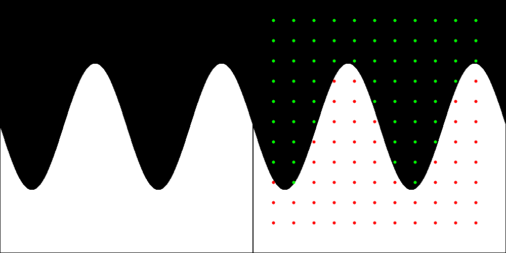
Fig 1: The sine wave image on the left is the original input image. The sine wave image on the right has a set of 121 sample points superimposed. The sample points that are coloured red were labelled with a class of “1”, while those that are green were labelled with a class of “0”.

A polynomial solution

A polynomial solution is the obvious “first try” when one thinks of attempting to “learn” a function that resembles a sine wave. The reason for this is that a sine wave can famously be decomposed into the following Taylor series:

This is a type of polynomial function. Where a polynomial function has the form:

Where $n$ is called the degree of the polynomial function, and the set $c_i$ is the set of coefficients, given that $0 \leq i < n$.

We can test our ability to fit a polynomial to a set of sampled points from the function $sin(x)$. The following Matlab code illustrates how this could be achieved:

% Setup the plot time axis
max = 2 * pi;
time_1 = 0 : 1 / 2e4 : max; % plot sample rate
time_2 = 0 : max / 20  : max; % selected sample rate

% Setup the wave and the sample wave
wave_1 = sin(time_1);
wave_2 = sin(time_2);

% Find the weights
A = [time_2', time_2.^3', time_2.^5', time_2.^7'];
B = [wave_2'];
C = A\B;

% Create an approximated wave using the coefficients
D = [time_1', time_1.^3', time_1.^5', time_1.^7'];
wave_3 = (D * C)';

% Plot the graph
hold on;
plot(time_1, wave_1);
plot(time_2, wave_2, 'o');
plot(time_1, wave_3);

This code attempts to fit the polygon of the form:

to the function $sin(x)$. Of course, these are only the first few terms of an infinite series, so we do not expect the result to be perfect - however, we expect the sine wave shape to be somewhat recognizable.

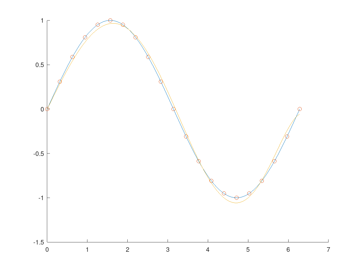
Fig 2: The plot produced by the Matlab code. The blue curve is the sine wave, the red circles indicate the locations of the sampled points, and the origin curve indicates the fitted polygon.

While this looks promising, this is not exactly what we are doing. If we refer back to Fig. 1, we are sampling a function $F$ with a two-dimensional input and a one-dimensional binary output. The sine wave is not directly sampled but is the shape of the boundary between the classes. It might be helpful to visualize the function in 3D space, as shown in Fig. 3. So while we know that a polynomial can reasonably approximate the boundary between classes of this function, the real question is whether it can infer this boundary from a sparse set of sample points taken at regular intervals over some defined region within the function $F$.

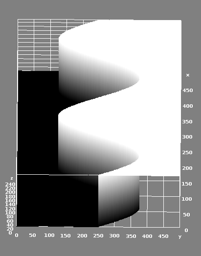
Fig 3: A 3D representation of the function that we are trying to learn. Strictly speaking, this image is incorrect because there are no "intermediate" points between the black and white regions - however, they make the image look pretty!

To try and test this, I attempted to approximate the function $F(x,y)$ with a 2D polynomial function $P(x,y)$. I arbitrarily selected nine terms such:

I used a pseudo-inverse to solve this, and based on a two-class fitting with labels “0” and “1”, I got an average error of $0.23 \pm 0.2$, which is not great.

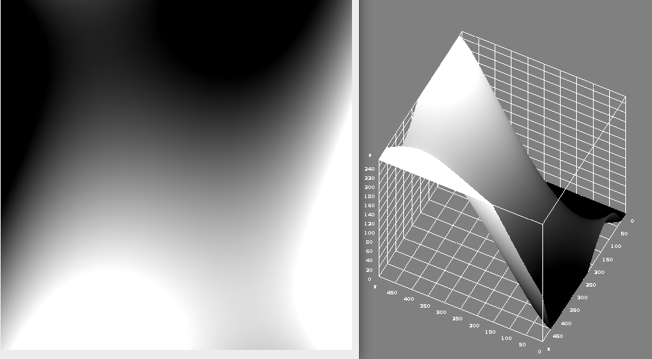
Fig 4: The poor fit can be visualized by rendering the output image as either 2D image (left) or a 3D image right.

While more time could have been spent trying out the various coefficient combinations, I ultimately felt that this approach was too limited to solve the tested problem and moved on to other techniques. I think that a strategy that focused on modelling the interface between both classes would have been far more effective, but structuring the learning problem this way focuses on the attributes of the problem itself, thus moving away from a general approach to machine learning.

A Support Vector Machine solution

Support Vector Machines (SVM) is a machine learning algorithm that became prominent in the 90s. While many variants exist, its primary form is a supervised learning algorithm that can be applied to discrete problems (classification) and continuous space problems (regression). SVM can be seen as a robust statistical learning approach that maps training data into n-dimensional space, such that it attempts to maximize the “gap” between various categories. A support vector machine can produce linearly separable models. However, non-linear models can also be achieved using the kernel trick [Link].

OpenCV contains an implementation of SVM in its machine learning module (ml.hpp). In our case, we can take our sample points and train our support vector machine as follows:

// Load points
auto points = vector<Vec3i>(); 
LoadPoints(input, points);

// Get Matrices
Mat A = GetDataMatrix(points);
Mat b = GetClassMatrix(points);

// Setup Terminator criteria
auto criteria = TermCriteria(TermCriteria::MAX_ITER, 1e4, 1e-6);
                        
// Create a Support Vector machine
Ptr<cv::ml::SVM> svm = cv::ml::SVM::create();
svm->setType(cv::ml::SVM::Types::C_SVC);
svm->setKernel(cv::ml::SVM::KernelTypes::INTER);
svm->setTermCriteria(criteria);

// Kick off the training
svm->train(A, cv::ml::ROW_SAMPLE, b);

We can then use this trained model to generate the image as follows:

// Build the resulting image
Mat image = Mat_<uchar>(500, 500);
for (auto row = 0; row < image.rows; row++) 
{
    for (auto column = 0; column < image.cols; column++) 
    {
        auto index = column + row * image.cols;
        Mat sampleMap = (Mat_<float>(1,2) << column, row);
        float response = svm->predict(sampleMap);
        
        if (response > 0.5) image.data[index] = 255;
        else image.data[index] = 0;
    }
}

Such an approach produces the following result (using the interpolation kernel option provided by OpenCV).

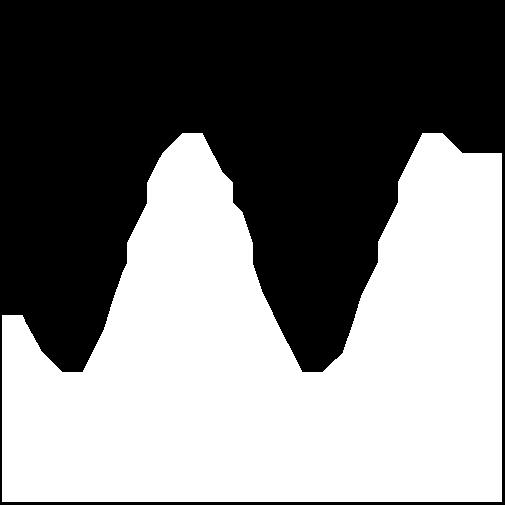
Fig 5: The resultant fit found using the SVM algorithm. Note from Fig. 1 that the right-hand position of the sine wave was not sampled, leading to the error on the right-hand side.

The choice of different kernels leads to different results. However, the interpolation kernel seemed the best choice for this particular task. The boundary between classes is a little jagged (compared to the ground-truth image), indicating some classification errors in the region between classes. However, generally, from this experiment, we can see that the SVM approach is a significant improvement in solving this problem when compared to the polynomial approach we looked at previously.

An Artificial Neural Network solution

The final approach we will look at is an artificial neural network (ANN) solution using the implementation packaged with the OpenCV API. ANN are biologically inspired networks of nodes and weights that encode mapping logic between a set of inputs and outputs. In the modern context, there are many different types of nodes; however, one of the oldest and most traditional nodes takes a set of inputs and “activates” (produces a non-zero output) when the sum of these inputs exceeds some sort of threshold. Such a node is known as a perceptron (see Fig. 6). A neural network is typically organized in layers, and a neural network constructed from multiple layers of perceptrons is known as a multi-layer perceptron artificial neural network.

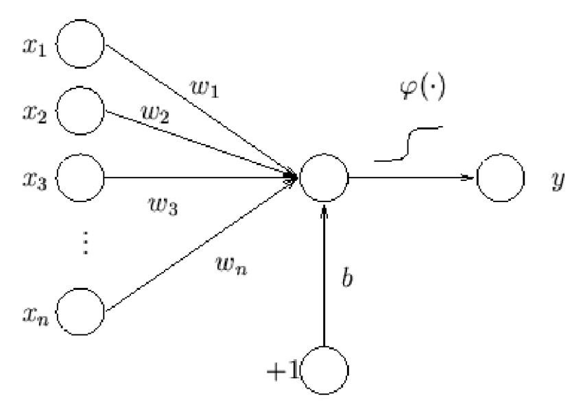
Fig 6: A graphical representation of a perceptron

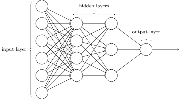
Fig 7: A depiction of a multi-layer perception artificial neural network.

To use such a system in OpenCV, we first need to define the structure of the network, which can be done as follows:

// Setup the neural network layer configuration
Mat_<int> layers(4,1);
layers(0) = 2;    // input
layers(1) = 100;  // hidden
layers(2) = 100;  // hidden
layers(3) = 1;    // output, 1 pin per class.

The next thing is to set up the neural network itself:

// Setup the network
Ptr<ml::ANN_MLP> network = ml::ANN_MLP::create();
network->setLayerSizes(layers);
network->setActivationFunction(ml::ANN_MLP::SIGMOID_SYM, 0, 0);
network->setTermCriteria(TermCriteria(
TermCriteria::MAX_ITER + TermCriteria::EPS, 100, 0.0001));
network->setTrainMethod(ml::ANN_MLP::BACKPROP, 0.0001);

Then training can commence!

Mat A = GetDataMatrix(points);
Mat b = GetClassMatrix(points);
Ptr<ml::TrainData> train =  ml::TrainData::create(A, ml::ROW_SAMPLE, b);

// Perform the initial training
network->train(train);

In my implementation, I have chosen to repeat the training loops 500 times, with each iteration refining the weights of the neural network further.

for (auto i = 0; i < 500; i++)
{
    cout << "Iteration: " << i << endl;
    network->train(train, ml::ANN_MLP::UPDATE_WEIGHTS);
    auto error = GetError(network, points);
    cout << "Error: " << error << endl;
}

Once the network is built, it can be used to predict outputs:

Mat sampleMap = (Mat_<float>(1, 2) << column, row);
Mat result = Mat_<float>(1, 1);
network->predict(sampleMap, result);

Given our toy problem, we get the following result:

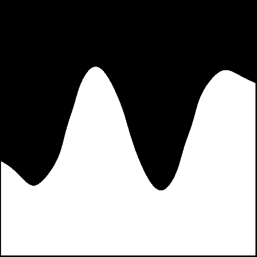
Fig 8: The result we obtained by training OpenCVs ANN MLP on the toy problem described at the beginning of this article.

Conclusions

This article looks at the tools that OpenCV 4 provides for fundamental machine learning operations. We defined a toy problem: to learn a simple 2D image depicting a dark-coloured region and light-coloured regions separated by a sine wave.

We first tried to solve this problem by basic polynomial fitting and found that our polynomial approach was insufficient. We then used OpenCV’s support vector machine and OpenCV’s multi-layer perceptron artificial neural network and found much better results.

The artificial neural network approach was the clear winner in this test, with the result surprisingly close to the original image, given the sparse sample of points provided as training data.