PatchMatch: Stereo Matching by Random Search

An interest of mine is extracting information from digital images. This is challenging because digital image data is usually stored on a computer as a massive array of color measurements (called pixels), which is not a particularly handy form if one wants to try and understand what is going on. One common way of making sense of image data is by fitting a model to the image data. Here, a model is some generalized abstract structure representing the information one wants to extract from the image, along with how this information relates to typical patterns of pixels expected to be found within the image. The role of the model is to impose meaning onto pixel clusters within the image, making it easier to work with.

So how does one go about fitting models to images? Well, this is typically framed as an optimization problem in which we define some “objective function” (say $f$) that measures how well a model (say $m$) fits with the image data. The model, in turn, is a flexible structure that can be adjusted to fit image data by tuning a set of parameters, say the vector $x$. Therefore given image $I$, we can measure the fit of a model $m$ as an error (say $\epsilon$) using the function $f$ such as

\[\epsilon = f(I, m(x))\]

The optimal set of model parameters $x^{\dagger}$ is the one that leads to the smallest possible residual $\epsilon^\dagger$, implying the best fitting model $m(x^\dagger)$.

There are many ways of finding optimal parameters, but one approach that has always fascinated me is random search. I have always thought there was something bold about skipping the whole part of trying to calculate the best solution and instead repeatedly selecting random numbers out of a hat and asking, “how about this one?”. Of course, unless the set of candidate solutions is relatively small, this will not lead to a reasonable solution in a hurry (unless you are super lucky). However, it can still be fun to try when you have time to spare, and it is sometimes an essential starting point if you don’t have much information about the “rules” of a new data space you need to search.

The stereo-matching problem

As the saying goes, a picture is worth a thousand words, which bears out with the immense diversity of information extraction problems associated with a field like Computer Vision (a specialization in Computer Science obsessed with replicating human visual system tasks on the computer). This article will focus on a problem known as the stereo-matching problem to make things tangible. Still, many of the ideas presented in this article can be generalized to address other types of information extraction problems, so the notions in this article don’t exclusively apply to stereo-matching.

The goal of stereo-matching is to extract the scene 3D geometry from images. When a camera captures a scene, it loses the depth dimension of scene data as it “converts” 3D scene elements $[X,Y,Z]^{\top}$ into 2D image measurements $[u,y]^{\top}$. This operation is equivalent to the mathematical operation known as a projection function. Projection functions are often non-invertible functions (the data discarded during the procedure cannot be regenerated to “undo” the operation). Unfortunately, this is very much the case with image projection. However, stereo-matching attempts to save the day by providing a way to guess at the missing $Z$ dimension using two images. Note that this approach is limited in accuracy and can be pretty error-prone since there often exists a lot of ambiguity in the recovery process.

At its core, stereo matching is about finding corresponding points (points across two images that measure a similar/identical 3D scene location). Corresponding pixels are helpful because they enable estimating depth $Z$, using the notion of triangulation.

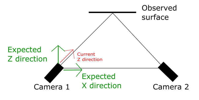
Fig 1: A graphical depiction of the “triangle” used in triangulation to acquire depth from a two-camera system.

Regarding the initial discussion, stereo-matching can also be considered a model-fitting problem. In this case, the model is a disjoint set of 3D surfaces parameterized by a discrete array of depth measurements, known as a depth map. The 3D location of each point of the surface model can be associated with 2D image locations by the projection models of each system camera. We can determine the quality of the fit by the consistency of colors of the corresponding points predicted by the surface (the same 3D point should have the same color [roughly] at each location of each of the images it is visible on - assuming a narrow baseline between images).

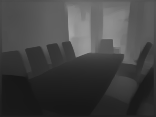
Fig 2: An example of a depth map. Each pixel represents the distance between the camera and the point in 3D space defined by the pixel. Close points are more black, while far points are more white.

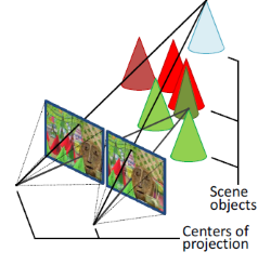
Fig 3: A depiction of corresponding points in a stereo-matching system. Corresponding points should have roughly the same color, but this could differ slightly due to measurement noise and different sensors in the case of multiple cameras.

Patch Match Stereo

Stereo-matching is a challenging problem. It is also a popular research topic because of its perception as an “important” problem. This “importance” comes from the belief that applications could (would?) benefit from the knowledge of 3D geometry - for example, robot navigation. Thus, many different approaches exist to approach solving its underlying optimization problem. It should come as no surprise that the current most effective strategies rely upon data-driven matching systems powered by the latest machine learning-developed models. However, “way back” in 2011, Bleyer et al. [1] released the Patch Match Stereo algorithm into the world. It was not the fastest algorithm, and the quality of the result it finds is average for its era (OpenCV preferred semi-global matching [2], for example). But the fact that it is a random search algorithm gave the Patch Match Stereo algorithm serious style points in my book!

You see, Patch Match Stereo begins with a randomly generated depth map - like, how cool is that?

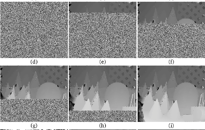
Fig 4: A few screenshots of the Patch Match Stereo algorithm in action per the master’s thesis of Kuang [3].

The use of random search itself is the basis of several machine learning and optimization algorithms, including swarm intelligence, genetic algorithms, and Monte Carlo methods. One way to think about random search is as an approach that repeatedly samples a problem space to gather statistics about that space. These statistics then support inferences that “hopefully” lead to a solution for the problem at hand.

The main benefits of a random search are:

• They can be very flexible regarding expected statistical distributions in the data. No “normal distribution” or “student distribution” is forced upon the data, and therefore the solutions can fit the problem a lot better than a solution with a predefined “shape.”
• They are general approaches applicable to a wide range of problems.
• They don’t impose a defined order on the search, which means that they can be highly effective in cases with a relatively commonly found uniform distribution of “good enough” solutions in the search space. (A systematic search is more focused on coverage, while a random search works well finding elements that are relatively typical in the search space)
• They tend to be relatively simple algorithms to implement and understand.
• Depending on the formulation, they don’t get “stuck” in local minima in the same way that algorithms that follow data gradients do.
• Search spaces often can be formulated intuitively for these types of algorithms rather than the more complex “black box” structures used for some more “state-of-the-art” approaches.

Random search has its problems too:

• The benefit that they are not tied that strongly to “prior knowledge” about the search space means that they tend to be far slower than algorithms that do exploit this knowledge.
• Compared to modern stochastic gradient-based approaches, they can be very slow.
• The random nature means they have unpredictable behavior unacceptable to a society that focuses on predictability, risk, and return.
• Many of these approaches are hard to parallelize, meaning that the hardware advancements driving the current artificial intelligence movement do not benefit these algorithms much.
• There is less hype around these algorithms than some of the more “mainstream” alternatives.
• In today’s world, more understandable search spaces are secondary to the primary goal of finding solutions for problems as quickly as possible.

The basic Patch Match algorithm

So how does the Patch Match algorithm work? As with a typical stereo-matching algorithm, the main goal is to fit a surface model to a pair of images. Now the standard parameterization of a surface model is a depth map (disparity map to be technical - but I am trying to avoid being too technical, and essentially a disparity map gets mapped to a depth map at some point anyway). However, the authors of the original Patch Match stereo algorithm used a more complex representation (slanted windows) to demonstrate the power of their new approach with a larger continuous search space than the standard discrete search space that is typical. This is understandable since it is hard to make a practical argument for their approach because “block matching” is just far simpler and essentially does the same thing. However, in my experience, I have applied the Patch Match algorithm directly to a depth map parameter space with good results, so the subsequent argument will be from the perspective of a depth map parameter space, even though that was not the original formulation.

So what properties of depth map parameter space are we trying to optimize? Well, the first observation is about the range of values. Recovering depth from a pair of images is only possible where corresponding points exist. Therefore the search for depth is limited to the region of overlap between the two images. Also, correspondence discovery is only effective when the corresponding points look similar. This can only occur when the two cameras are sufficiently close to each, called “the narrow baseline assumption.”

Consequently, there is a minimum natural depth below which no corresponding points exist between cameras. Also, as points are further away from the camera, the depth resolution deteriorates (increases) at a quadratic rate (due to perspective projection, closer objects have higher resolution than objects future away). This usually leads to a natural upper depth limit (beyond which the likely depth error is too large for the application to function correctly). Thus, the depth values we are looking for are usually constrained to some range, and it is often not an extensive range (in terms of pixels) due to the quadratic deterioration.

Fig 5: A photograph normally exhibits perspective projection, meaning that things close to the camera appear bigger (have more pixels and therefore a high resolution) than things of the same size further away from the camera.

Another property of depth maps is that they usually depict scenes containing a set of objects. All pixels (except for noise) are measurements from object surfaces (where the light reflects off for image generation). Object surfaces are smooth structures (even rough objects because there is still some connectivity between neighboring pixels), implying that pixels and their neighbors probably have similar values.

Thus we have a scenario in which a depth map of random values will probably have a portion estimates reasonably close to the optimal value due to the relatively small range sampled. Patch Match Stereo then introduces the idea of propagation, meaning that depths with a better-fit score replace weaker depth values. Propagation occurs from potential sources of suitable values for a given pixel (neighbors, corresponding views, and previous video sequence frames). Finally, there is a random refinement stage that proposes possible minor improvements to each depth value with the goal of fine-tuning. And that is the algorithm!

My Implementation

My interest has been in the characteristics of random search in this problem space.

Therefore, the main focus of my implementation was to attempt to generalize the proposed refinement propagations proposed in the original work. I spent little time on the actual cost function (evaluating fit). Thus, I used nothing more sophisticated than a simple block-matching approach after establishing that straight pixel-based matching produced very noisy results.

I managed to reduce the “propagations” of good values down to two operations:

• A local optimization: Randomly select a neighbor to the pixel in question, and determine whether the depth associated with the neighbor is an improvement.
• A refinement optimization: Randomly modify the pixel depth with a minor update (positive or negative) and see if that leads to an improvement.

With these two refinements in place, I found that my algorithm converged to a solution almost as quickly as the original formulation (within a few iterations) with a typical optimization graph shape (a fast initial improvement that slows down as the solution approaches the optimum). I have attached the graph below:

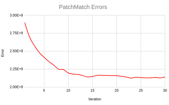
Fig 6: The graph of the improvement of the block matching score as the depth map is refined to fit a stereo pair. The error is the total error across the entire image (168750 pixels). I ran the algorithm over 30 iterations.

The main test image used in this experiment was the classic “teddy” from the 2003 images available on the Middlebury Stereo website. As far as stereo matching is concerned, this image is only a simple challenge. Subsequent Middlebury datasets from later years are far more challenging. However, my goal was to get a feel for the algorithm, not put it through its paces (yet).

Fig 7: The “left” image from the Middlebury stereo dataset

The result of a typical run against the “teddy” image can be seen below. I have implemented far more sophisticated cost functions in the past and got far better-looking results. Also, I have not attempted to remove occlusions from the result (an occlusion is a pixel visible in only one image of the stereo pair, which tends to be the most obvious at the edge of a foreground object, like a chimney). However, my main focus has been on the ability of the algorithm to converge toward a solution, which I claim I did successfully. The quality of the solution is a topic for a future article.

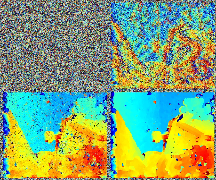
Fig 8: A sequence of depth maps as the algorithm converges towards its solution. In the first frame is the initial random depth map. The next frame is the improvement after 1 iteration. The frame next to that is after ten iterations. The final frame is after 30 iterations.

Future Work

This work was an initial investigation into Patch Match Stereo to become familiar with the algorithm after a long absence. I now aim to investigate its use as a solution for multi-view stereo problems, which is not a novel idea (see [4]). However, despite the lack of novelty, I still think it could be a valuable tool for creating and improving high-quality, large-scale 3D models.

References

1. M. Bleyer, C. Rhemann, and C. Rother, “Patchmatch stereo-stereo matching with slanted support windows,” in Bmvc, vol. 11, pp. 1–11, 2011.
2. H. Hirschmuller, “Accurate and efficient stereo processing by semi-global matching and mutual information,” in 2005 IEEE Computer Society Conference on Computer Vision and Pattern Recognition (CVPR’05), vol. 2, pp. 807–814, IEEE, 2005.
3. F. Kuang, “Patchmatch algorithms for motion estimation and stereo reconstruction,” in Master’s thesis, University of Stuttgart, 2017.
4. H. Song, J. Park, S. Kang, J. Lee, “Patchmatch based multiview stereo with local quadric window,” Proceedings of the 28th ACM International Conference on Multimedia. 2020.